Model-Free Prediction
One of the problems with DP is that it assumes full knowledge of the MDP, and consequently, the environment. While this holds true for a lot of applications, it might not hold true for all cases. In fact, the upper limit does turn out to be the ability to be accurate about the underlying MDP. Thus, if we don’t know the true MDP behind a process, the next best thing would be to try to approximate them. One of the ways to go about this is Model-Free RL.
Monte-Carlo Methods
The core idea behind the Monte-Carlo approach, which has its root in gambling, is to use probability to approximate quantities. Suppose we have to approximate the area of a circle relative to a rectangle inside which it is inscribed (This is a classic example and an easy experiment), the experiment-based approach would be to make a board and randomly throw some balls on it. In a true random throw, let’s call the creation of a spot on the board a simulation ( experiment, whatever!). After each simulation, we record the number of spots inside the circular area and the total number of spots including the circular area and the rectangular area. A ratio of these two quantities would give us an estimate of the relative area of the circle and the rectangle. Now as we conduct more such experiments, this estimate would actually get better since the underlying probability of a spot appearing inside the circle is proportional to the amount of area that the circle occupies inside the rectangle. Hence, if we keep doing this our approximation gets increasingly closer to the true value.
Applying MC idea to RL
Another way to put the Monte-Carlo approach would be to say that Monte-Carlo methods only require experience. In the case of RL, this would translate to sampling sequences of states, actions, and rewards from actual or simulated interaction with an environment. An experiment in this sense would be a full rollout of an episode which will create a sequence of states and rewards. When multiple such experiments are conducted, we get better approximations of our MDP. To be specific, our goal here would be to learn \(v_{\pi}\) from the episodes under policy \(\pi\). The value function is the expected reward:
\[v_{\pi}(s)= \mathbb{E}_{\pi}[G_t∣S_t=s]\]So, all we have to do is estimate this expectation using the empirical mean of the returns for the experiments
First-Visit MC Evaluation
To evaluate state s, at the first time-step t at which s is visited:
- Increment counter: \(N(s) \leftarrow N(s) + 1\)
- Increment total return: \(S(s) \leftarrow S(s) + 1\)
- Estimate value by the mean return: \(V(s) = \frac{S(s)}{N(s)}\)
As we repeat more experiments and update the values at the first visit, we get convergence to optimal values i.e \(V(s) \rightarrow v_{\pi}\) as \(N(s) \rightarrow \infty\)
Every-Visit MC Evaluation
This is same as first visit evaluation, except we update at every visit:
- \[N(s) \gets N(s) + 1\]
- \[S(s) \gets S(s) + 1\]
- \[V(s) = \frac{S(s)}{N(s)}\]
Incremental MC updates
The empirical mean can be expressed as an incremental update as follows:
\[\begin{aligned} \mu_k &= \frac{1}{k} \sum_{j=1}^n x_j \\ &= \frac{1}{k} (x_k + \sum_{j=1}^{k-1} x_j) \\ &= \frac{1}{k} (x_k + (k-1)\mu_{k-1}) \end{aligned}\]Thus, for the state updates, we can follow a similar pattern, and for each state \(S_t\) and return \(G_t\), express it as:
- \[N(S_t) \gets N(S_t) + 1\]
- \[(S_t) = V(S_t) + \frac{1}{N(S_t)}(G_t - V(S_t))\]
Another useful way would be to track a running mean:
\[V(S_t) \gets V(S_t) + \alpha (G_t - V(S_t)\]Temporal-Difference (TD) Learning
The MC method of learning needs an episode to terminate in order to work its way backward. In TD, the idea is to work the way forward by replacing the remainder of the states with an estimate. This is one method that is considered central and novel to RL (According to Sutton and Barto). Like MC methods, TD methods can learn directly from raw experience, and like DP, TD methods update estimates based in part on other learned estimates, without waiting for a final outcome, something which is called Bootstrapping - updating a guess towards a guess (meta-guess-update?).
Concept of Target and Error
If we look at the previous equation of Incremental MC, the general form that can be extrapolated is
\[V(S_t) \gets V(S_t) + \alpha (T - V(S_t)\]Here, the quantity \(T\) is called the Target and the quantity \(T - V(S_t)\) is called the error. In the MC version, the target is the return \(G_t\), which means that the MC method has to wait for this return to be propagated backward to see the error of its current value function from this return, and improve. This is where TD methods show their magic; At time \(t+1\), they can immediately form a target and make a useful update using the observed reward and the current estimate of the value function. The simplest TD method, \(TD(0)\), thus has the following form:
\[V(S_t) \gets V(S_t) + \alpha (R_{t+1} + \gamma V(S_{t+1}) - V(S_t))\]This is why bootstrapping is a guess of guess, since the TD method bases its update in part on an existing estimate.
Comparing TD, MC and DP
Another way to look at these algorithms would be through the Bellman optimality equation:
\[v_{\pi}(s) = E [ R_{t+1} + \gamma v_{\pi}(S_{t+1})| S_t = s]\]which allows us to see why certain methods are estimates:
- The MC method is an estimate because it does not have a model of the environment and thus, needs to sample in order to get an estimate of the mean.
- The DP method is an estimate because it does not know the future values of states and thus, uses the current state value estimate in its place.
- The TD method is an estimate because it does both of these things. Hence, it is a combination of both. However, unlike DP, MC and TD do not require a model of the environment. Moreover, the online nature of these algorithms is something that allows them to work with samples of backups, whereas DP requires full backup.
TD and MC can further be differentiated based on the nature of the samples that they work with:
- TD requires shallow backups since it is inherently online in nature
- MC requires deep backups due to the nature of its search.
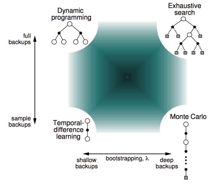
Another way to look at the inherent difference is to realize that DP inherently does a breadth-first search, while MC does a depth-first search. TD(0) only looks one step ahead and forms a guess. These differences can be summarized on the following spectrum by David Silver, which I find really helpful:

Extending TD to n-steps
The next natural step for something like TD would be to extend it to further steps. For this, we generalize the target and define it as follows:
\[G^{(n)}_t = R_{t+1} + \gamma R_{t+2} + ... + \gamma^{n-1} R_{t+ n} + \gamma^n V(S_{t+n}))\]And so, the equation again follows the same format:
\[V(S_t) \gets V(S_t) + \alpha (G^{(n)}_t - V(S_t)\]One interesting thing to note here is that if the value of \(n\) is increased all the way to the terminal state, then we essentially get the same equation as MC methods!
Averaging over n returns
To get the best out of all the \(n\) steps, one improvement could be to average the returns over a certain number of states. For example, we could combine 2-step and 4-step returns and take the average :
\[G_{avg} = \frac{1}{2} [ G^{(2)} + G^{(4)} ]\]This has been shown to work better in many cases, but only incrementally.
\(\lambda\)-Return → Forward View
This is a method to combine the returns from all the n-steps:
\[G^{(\lambda)}_t = (1 - \lambda ) \displaystyle\sum_{n=1}^{\infin} \lambda^{n-1} G^{(n)}_t\]And this, is also called Forward-view \(TD(\lambda)\).
Backward View
To understand the backward view, we need a way to see how we are going to judge the causal relationships between events and outcomes (Returns). There are two heuristics:
- Frequency Heuristic → Assign credit to the most frequent states
- Recency Heuristic → Assign credit to the most recent states.
The way we keep track of how each states fares on these two heuristics is through Eligibility Traces:
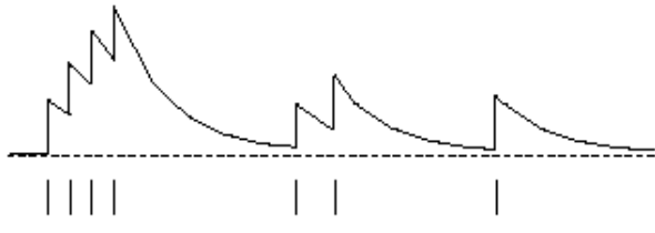
\[E_t(s) = \gamma \lambda E_{t-1}(s) + \bold{1}(S_t = s)\]These traces accumulate as the frequency increases and are higher for more recent states. If the frequency drops, they also drop. This is evident in the figure below:

So, all we need to do it scale the TD-error \(\delta_t\) according to the trace function:
\[V(S) \gets V(S) + \alpha \delta_t E_t(s)\]Thus, when \(\lambda = 0\), we get the equation for \(TD(0)\) , and when \(\lambda =1\), the credit is deferred to the end of the episode and we get MC equation.