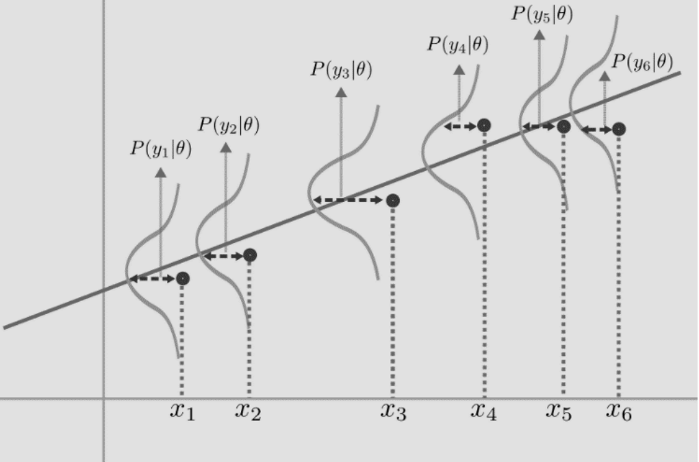
Maximum Likelihiood Estimation
Main Idea:
- Make an explicit assumption about what distribution the data was modeled from
- Set the parameters of this distribution so that the data we observe is most likely i.e maximize the likelihood of our data
For a simple example of a coin toss, we can see this as maximizing the probability of observing heads from a binomial distribution:
\[p(z_1, ..., z_n) = p(z_1 ...., z_n|\theta)\]we assume I.I.D condition and so we should be able to break this down into :
\[p(z_1|\theta)p(z_2|\theta)....p(z_n|\theta)\]Formally, let us deinfe a likelihood function as:
\[L(\theta) = \prod_{i=1}^N p(z_i|\theta)\]Now, our task it to find the \(\hat{\theta}\) that maximizes this likelihood:
\[\hat{\theta}_{MLE} = \underset{\theta}{\text{argmax}} \prod_{i=1}^N p(z_i|\theta)\]instead of maximizing a product, we can also view this problem as minimizing a sum if we take the log of all values:
\[\hat{\theta}_{MLE} = \underset{\theta}{\text{argmax}} \sum_{i=1}^N Log(p(z_i|\theta))\]Let us use this idea for the regression problem. We assume that our outputs are distributed in a Gaussian manner around the line w have to find out. This basically means that our \(\epsilon\) is a Gaussian Noise that is messing up our outputs from the fundamental distribution

Thus, our equation for getting this probability of our output would be :
\[p(y_i|x_i; w_i, \sigma^2) = \frac{1} {\sigma \sqrt {2\pi } } exp\{ \frac{ - (y_i - x_iw)^2 }{2 \sigma^2} \}\]Our task is to estimate \(\hat{w}\) such that the likelihood of \(p\) is maximized. This, in other words, means we need to find the value of \(w\) that maximizes the above expression:
\[\begin{aligned} & \hat{w} = \underset{w}{\text{argmax}} \prod_{i=1}^N p(y_i|x_i; w_i, \sigma^2) \\ \implies & \hat{w} = \underset{w}{\text{argmax}} \prod_{i=1}^N \frac{1} {\sigma \sqrt {2\pi } } exp\{ \frac{ - (y_i - x_iw)^2 }{2 \sigma^2} \} \end{aligned}\]we can again do the log trick to make this a sum maximization :
\[\begin{aligned} &\hat{w} = \underset{w}{\text{argmax}} \sum_{i=1}^N Log(\frac{1} {\sigma \sqrt {2\pi } } exp\{ \frac{ - (y_i - x_iw)^2 }{2 \sigma^2} \}) \\ \implies &\hat{w} = \underset{w}{\text{argmax}} \{ \sum_{i=1}^N Log(\frac{1}{\sigma \sqrt {2\pi}}) + \sum_{i=1}^N Log(exp\{ \frac{ - (y_i - x_iw)^2 }{2 \sigma^2} \}) \} \\ \implies &\hat{w} = \underset{w}{\text{argmax}} -\sum_{i=1}^N \frac{(y_i - x_iw)^2}{2 \sigma^2} \end{aligned}\]This is basically the same as the normal expression we had, the only difference being the normalizing factor \(\sigma\). If we change the negative maximization to minimization:
\[\hat{w} = \frac{1}{2 \sigma^2} \underset{w}{\text{argmin}} \sum_{i=1}^N (y_i - x_iw)^2\]Which is the same as minimizing :
\[\hat{w} = \underset{w}{\text{argmin}} \sum_{i=1}^N (y_i - x_iw)^2\]and the solution is:
\[\mathbf{w} = (\mathbf{X}^T\mathbf{X})^{-1} \mathbf{X}^T\mathbf{y}\]Surprise, Surprise!!