Markov Processes
These are random processes indexed by time and are used to model systems that have limited memory of the past. The fundamental intuition behind Markov processes is the property that the future is independent of the past, given the present. In a general scenario, we might say that to determine the state of an agent at any time instant, we only have to condition it on a limited number of previous states, and not the whole history of its states or actions. The size of this window determines the order of the Markov process.
To better explain this, one primary point that needs to be addressed is that the complexity of a Markov process greatly depends on whether the time axis is discrete or topological. When this space is discrete, then the Markov process is a Markov Chain. A basic level understanding of how these processes play out in the domain of reinforcement learning is very clear when analyzing these chains. Moreover, the starting point of analysis can be further simplified by limiting the order of Markov Processes to first-order. This means that at any time instant, the agent only needs to see its previous state to determine its current state, or its current state to determine its future state. This is called the Markov Property
\[\mathbb{P}(S_{t+1}|S_t) = \mathbb{P}(S_{t+1}|S_1, ..., S_t) )\]Markov Process
The simplest process is a tuple \(<S,P>\) of states and Transitions. The transitions can be represented as a Matrix \(P = [P_{ij}]\), mapping the states - \(i\) - from which the transition originates, to the states - \(j\) - to which the transition goes.
\[\begin{bmatrix} P_{11} & . & . & . & P_{1n}\\ . & . & . & . & . \\ . & . & . & . & . \\ . & . & . & . & . \\ P_{n1} & . & . & . & P_{nn} \end{bmatrix}\]Another way to visualize this would be in the form of a graph, as shown below, courtesy of David Silver.
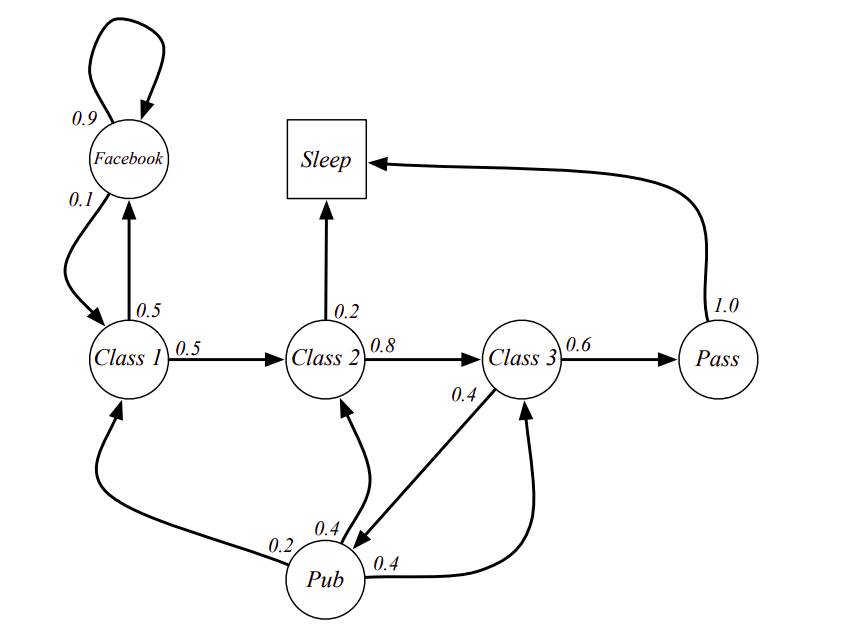
This is a basic chain that represents the actions a student can take in the class, with associated probabilities of taking those actions. Thus, in the state - Class 1 - the student has an equal chance of going to the next class or browsing Facebook. Once they start browsing Facebook, then they have a 90% chance of continuing to browse since it is addictive. Similarly, other states can be seen too.
Markov Reward Process
Now if we add another parameter of rewards to the Markov processes, then the scenario changes to the one in which entering each state has an associated expected immediate reward. This, now, becomes a Markov Reward Process.
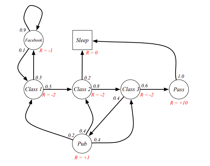
To fully formalize this, one more thing that needs to be added is the discounting factor \(\gamma\). This is a hyperparameter that represents the amount of importance we give to future rewards, something like a ‘shadow of the future’. The use of Gamma can be seen in computing the return \(G_t\) on a state:
\[G_t = R_{t+1} + \gamma R_{t+2} + \gamma^2 R_{t+3} + ...\]The reasons for adding this discounting are:
- To account for uncertainty in the future, and thus, better balance our current decisions → The larger the value, the more weightage we give to the ‘shadow of the future’
- To make the math more convenient → only when we discount the successive terms, we can get convergence on an infinite GP
- To avoid Infinite returns, which might be possible in loops within the reward chain
- This is similar to how biological systems behave, and so in a certain sense, we are emulating nature.
Thus, the reward process can now be characterized by the tuple \(<S, P, R, \gamma >\) . To better analyze the Markov chain, we will also define a way to estimate the value of a state - Value function - as an expectation of the Return on that state. Thus,
\[V(S) = \mathbb{E} [ G_t| S_t = s ]\]An intuitive way to think about this is in terms of betting. Each state is basically a bet that our agent needs to make. Thus, the process of accumulating the rewards represents the agent’s understanding of each of these bets, and to qualify them, the agent has to think in terms of the potential returns that these bets can give. This is what we qualify here as the expectation. But the magic comes when we apply it recursively, and this is called the Bellman Equation
\[V(S) = \mathbb{E} [R_{t+1} + \gamma V(S_{t+1}| S_t = s]\]This equation signifies that the value of the current state can be seen in terms of the value of the next state and so on, and thus, we can have a correlated relationship between states. To better see how this translates to the whole chain, we can also express this as a Matrix Operation:
\[\begin{bmatrix} V_1 \\ . \\ . \\ V_n \end{bmatrix} = \begin{bmatrix} R_1 \\ . \\ . \\ R_n \end{bmatrix} \begin{bmatrix} P_{11} & . & . & P_{1n}\\ . & . & . & . \\ . & . & . & . \\ P_{n1} & . & . & P_{nn} \end{bmatrix} \begin{bmatrix} V_1 \\ . \\ . \\ V_n \end{bmatrix}\]And so, the numerical way to solve this would be to invert the matrix (assuming it is invertible) and the solution, then would be:
\[\bm{\bar{V}} = (1 - \gamma \bm{\bar{P}})^{-1} \bm{\bar{R}}\]However, as anyone familiar with large dimensions knows, this becomes intractable pretty easily. Hence, the whole of RL is based on figuring out ways to make this tractable, using majorly three kinds of methods:
- Dynamic Programming
- Monte-Carlo Methods
- Temporal Difference Learning
Markov Decision Process
If we add actions to the Markov Reward Process, then there can multiple states that the agent can reach by taking action to each state. Thus, the agent now has to decide which action to take. This is called a Markov Decision Process.
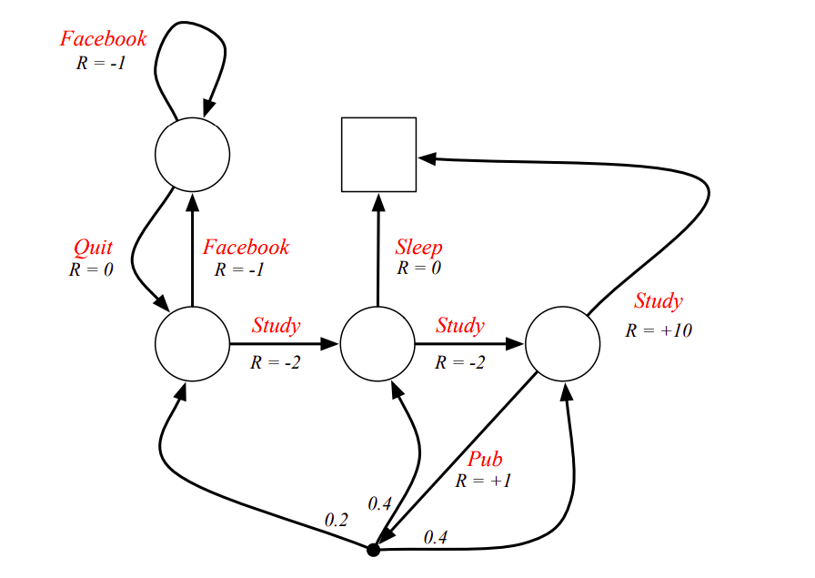
Thus, the MDP can be summarized by the tuple \(<S, A, P, R, \gamma >\). Here, we can also define the transitions and rewards in terms of the actions:
\[\begin{aligned} R^{a}_s &= \mathbb{E}[ R{t+1} | S_t=s, A_t=a ] \\ P^{a}_{ss'} &= \mathbb{P}[ S{t+1}=s'| S_t=s, A_t=a ] \end{aligned}\]Now, the important thing is how the agent makes these decisions. The schema that the agent follows for this is called a Policy, which can be seen as the probability of taking an action, given the state:
\[\pi (a|s) = \mathbb{P} [ A_t = a | S_t = s ]\]Under a particular policy \(\pi\), the Markov chain that results is nothing but an MRP, since we don’t consider the actions that the agent did not take. This can be characterized by \(<S, P^{\pi}, R^{\pi}, \gamma>\), and the respective transitions and rewards can be described as:
\[\begin{aligned} R^{\pi}_{s} &= \sum_{\substack{a \in A}} \pi (a|s) R^{a}_{s}\\ P^{\pi}_{ss'} &= \sum_{a \in A} \pi (a|s) P^{a}_{ss'} \end{aligned}\]Another important thing that needs to be distinguished here is the value function, which can be defined for both states and actions:
-
State-Value Function (\(v_{\pi}\)): Values for states when policy \(\pi\) is followed
\[v_{\pi}(s) = \mathbb{E}_{\pi}[G_t | S_t = s]\] -
Action-Value Function (\(q_{\pi}\)): Expected return on starting from state \(s\), following policy \(\pi\), and taking action \(a\)
\[q_{\pi}(s, a) = \mathbb{E}_{\pi}[G_t | S_t = s, A_t = a]\]
Bellman Equation for MDPs
We can extend the bellman formulation to recursively define the qualities of state and actions:
\[\begin{aligned} &v_{\pi}(s) = \mathbb{E}_{\pi} \big[R_{t+1} + \gamma v_{\pi}(s')| S_t = s, S_{t+1} = s'\big] \\ &q_{\pi}(s, a) = \mathbb{E}_{\pi} \big[R_{t+1} + \gamma q_{\pi}(s', a')| S_t = s, S_{t+1} = s', A_t = a, A_{t+1} = a' \big] \end{aligned}\]However, a better way is to look at the inter-dependencies of these two value functions. The value of the state can be viewed as the sum of the value of the actions that can be taken from this state, which can, in turn, be viewed as the weighted sum of values of the states that can result from each action.
The expectation for the value of the states is the sum of the values of the actions that can result from that state
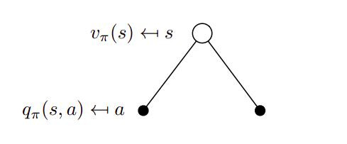
Thus, under the policy \(\pi\) this value is the sum of the q-values of the actions:
\[v_{\pi}(s) = \sum_{a \in A} \pi (a|s) q_{\pi} (s,a)\]Now, the action can be viewed in a similar manner as a sum over the value fo the states that can result from it
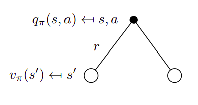
and written in the same manner
\[q_{\pi}(s,a) = R^{a}_s + \gamma \sum_{s' \in S} P^{a}_{ss'} v_{\pi} (s)\]And, if we put these equations together, we can get a self-recursive formulation of the bellman expectation equation. Thus, for the state this would be
\[v_{\pi}(s) = \sum_{a \in A} \pi (a|s) [ R^{a}_s + \gamma \sum_{s' \in S} P^{a}_{ss'} v_{\pi} (s) ]\]A Visualization for this would basically be a combination of the above two trees
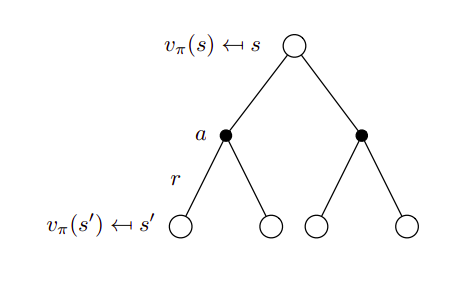
A similar process can be done for the action value function, and the result comes out to be
\[q_{\pi}(s,a) = R^{a}_s + \gamma \sum_{s' \in S} P^{a}_{ss'} \sum_{a' \in A} \pi (a'|s') q_{\pi} (s',a')\]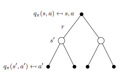
Bellman Optimality Equation
With the recursive forms, the question really comes on how do we go about creating a closed-loop optimality criterion. Here, the key point that needs to be taken into account is The agent is free to choose the action that it can take in each state, but it can’t choose the state that results from that action. This means, we start from a state, and maximize the result by choosing the action with the maximum action value. This is the first step of lookahead. Now, each of those actions has the associated action value that needs to be determined. In the case where the action can only lead to one state, it’s all well and good. However, in the case where multiple states can result out of the action, the value of the action can be determined by basically rolling a dice and seeing which state the action leads to. Thus, the value of the state that the action leads to determines the value of the action. This happens for all the possible actions from our first state, and thus, the value of the state is determined. Hence, with this Two-step lookahead, we can formulate the decision as maximizing the action values.
\[v_{\pi}(s) = \max_{a} \{ R^{a}s + \gamma \sum_{s' \in S} P^{a}_{ss'} v{} (s) \}\]Now, the question arises as to how can this equation be solved. The thing to note here is the fact that it is not linear. Thus, in general, there exists no closed-form solution. However, a lot of work has been done in developing iterative solutions to this, and the primary methods are:
- Value Iteration: Here methods solve the equation by iterating on the value function, going through episodes, and recursively working backward on value updates
- Policy Iteration: Here, the big idea is that the agent randomly selects a policy and finds a value function corresponding to it. Then it finds a new and improved policy based on the previous value function, and so on.
- Q Learning: This is a model-free way in which the agent is guided through the quality of actions that it takes, wit the aim of selecting the best ones
- SARSA: Here the idea is to iteratively try to close the loop by selecting a State, Action, and Reward and then seeing the State and Action that follows.
Extensions to MDP
MDPS, as a concept, has been extended to make them applicable to multiple other kinds of problems that could be tackled. Some of these extensions are:
- Infinite and Continuous MDPs: In this extension, the MDP concept is applied to infinite sets, mainly countably infinite state or action spaces, Continuous Spaces (LQR), continuous-time et. al
- Partially Observable MDPs (POMDP): A lot of scenarios exist where there are limits on the agent’s ability to fully observe the world. These are called Partially-Observable cases. Here, the state is formalized in terms of the belief distribution over the possible observations and encoded through the history of the states. The computations become intractable in theory, but many interesting methods have been devised to get them working. Eg. DESPOT
- Undiscounted and Average Reward MDP: These are used to tackle ergodic MDPs - where there is a possibility that each state can be visited an infinite number of times ( Recurrence), or there is no particular pattern in which the agent visits the states (Aperiodicity) - and to tackle this, the rewards are looked at as moving averages that can be worked with on instants of time.